FAB p-values for a hidden Markov model

Summary

This is a simulation study in which adaptive FAB \(p\)-values are constructed using a Gaussian hidden Markov model as a linking model. A binary hidden Markov model is the “true” linking model. This document serves as the replication code for the example in Section 3.4 of the article “Smaller \(p\)-values via indirect information” (Hoff 2019).

Here are some \(p\)-value functions:

#### ---- p-value functions

## -- FAB p-values
pFAB<-function(y,sigma,etheta=0,vtheta=1){
  c(1-abs( pnorm( (y+2*etheta*sigma^2/vtheta)/sigma ) - pnorm(-y/sigma) ))
}

## -- UMPU p-values
pUMPU<-function(y,sigma){
  c(2*pnorm(-abs(y)/sigma ))
}

## -- BH FDR control procedure
rejectBH<-function(pvals,fdr=.1){
  pc<-cbind(sort(pvals),fdr*(1:length(pvals))/length(pvals))
  nd<-max( c(0, suppressWarnings(which(pc[,1]<pc[,2])) ) )
  order(pvals)[seq(1,nd,length=nd)]
}

Here is a function that estimates the parameters in the linking model:

## -- mle from Gaussian hidden Markov model 
mleGHMM<-function(y){
  suppressWarnings( fit<-arima(y,c(1,0,1)) )

  ## TSA4 page 98
  phi<-fit$coef[1] ; theta<-fit$coef[2] ; mu<-fit$coef[3]
  sw2<-fit$sigma2

  v<-sw2*(1+2*theta*phi+theta^2)/(1-phi^2)
  w<-(1+theta*phi)*(theta+phi)/( phi*(1+2*theta*phi+theta^2)  )
  rho<-phi

  sigma2<-v*(1-w)
  psi2<-v*w

  x<-c(sigma2,mu,psi2,rho)
  names(x)<-c("sigma2","mu","psi2","rho")

  gam<-c(x[2]*(1-x[4]),x[4],sqrt(x[3]*(1-x[4]^2)),sqrt(x[1]))
  names(gam)<-c("beta0","beta1","tau","sigma")
  gam
}

Here is a function that computes an estimated conditional expectation and variance for the mean at location \(j\) given the data at the other locations:

## -- function to find conditional mean under linking spatial regression model 
cdistGHMM<-function(beta0,beta1,tau,sigma,r){
  w<-2*r+1
  d<-abs(outer(1:w,1:w,"-"))
  C<-(beta1^d)*tau^2/(1-beta1^2)
  iC<-solve(C)
  G<-diag(w)[-(r+1),]
  V<-solve( iC+t(G)%*%G/sigma^2 )
  b0<-c(V%*%( iC%*%(rep(beta0/(1-beta1),w)   ) ))[r+1]
  b1<-(V%*%t(G)%*%G)[r+1,]/sigma^2

  list(b0=b0,b1=b1,vtheta=V[r+1,r+1])
}

Here is the simulation study:

#### ---- HMM parameters 
TP<-rbind( c(.975,.025,.0), c(.01,.99,.01), c(0,.025,.975))
sigma<-1


#### ---- other parameters 
p<-1000
fdr<-.2
r<-50


#### ---- simulation study
EFAB<-XFAB<-UMPU<-pXNULL<-NULL

for(s in 1:100){

  #### ---- generate data
  set.seed(s) 
  theta<-0
  for(j in 2:p){theta<-c(theta,sample(c(-1,0,1),1,prob=TP[theta[j-1]+2,])) } 
  y<-rnorm(p,theta,sigma)

  #### ---- UMPU p-values 
  pU<-pUMPU(y,sigma)
  dU<-rejectBH(pU,fdr) 
  UMPU<-rbind(UMPU,c( sum(theta[setdiff(1:p,dU)]==0), sum(theta[dU]==0),
                      sum(theta[setdiff(1:p,dU)]!=0), sum(theta[dU]!=0) ) )

  #### ---- obtain eBayes means using single estimate of HMM params
  hmm<-mleGHMM(y)
  pripar<-cdistGHMM(hmm[1],hmm[2],hmm[3],hmm[4],r) 
  etheta<-NULL
  for(i in 1:p){
    ii<-seq(i-r,i+r) ; ii[ii<1]<-1 ; ii[ii>p]<-p
    etheta<-c(etheta, pripar$b0 + sum(pripar$b1*y[ii])  )
  }
  pX<-pFAB(y,sigma,etheta,pripar$vtheta)
  dX<-rejectBH(pX,fdr)
  XFAB<-rbind(XFAB,c( sum(theta[setdiff(1:p,dX)]==0), sum(theta[dX]==0),
                      sum(theta[setdiff(1:p,dX)]!=0), sum(theta[dX]!=0) ) ) 
  pXNULL<-c(pXNULL,pX[theta==0] )


  #### ----- exact FAB p-values
  mstheta<-NULL
  for(i in 1:p){ 
    ymi<-replace(y,i,NA)  
    if(i==1){ ymi<-ymi[-1] } 
    if(i==p){ ymi<-ymi[-p] } 
    hmm<-mleGHMM(ymi) 
    pripar<-cdistGHMM(hmm[1],hmm[2],hmm[3],hmm[4],r)
    ii<-seq(i-r,i+r) ; ii[ii<1]<-1 ; ii[ii>p]<-p 
    mstheta<-rbind(mstheta,c(pripar$b0 + sum(pripar$b1*y[ii]),pripar$vtheta ))
  }
  pF<-pFAB(y,sigma,mstheta[,1],mstheta[,2])
  dF<-rejectBH(pF,fdr)
  EFAB<-rbind(EFAB,c( sum(theta[setdiff(1:p,dF)]==0), sum(theta[dF]==0), 
                      sum(theta[setdiff(1:p,dF)]!=0), sum(theta[dF]!=0) )  )
  cat(s,"\n")  
}

## 1 
## 2 
## 3 
## 4 
## 5 
## 6 
## 7 
## 8 
## 9 
## 10 
## 11 
## 12 
## 13 
## 14 
## 15 
## 16 
## 17 
## 18 
## 19 
## 20 
## 21 
## 22 
## 23 
## 24 
## 25 
## 26 
## 27 
## 28 
## 29 
## 30 
## 31 
## 32 
## 33 
## 34 
## 35 
## 36 
## 37 
## 38 
## 39 
## 40 
## 41 
## 42 
## 43 
## 44 
## 45 
## 46 
## 47 
## 48 
## 49 
## 50 
## 51 
## 52 
## 53 
## 54 
## 55 
## 56 
## 57 
## 58 
## 59 
## 60 
## 61 
## 62 
## 63 
## 64 
## 65 
## 66 
## 67 
## 68 
## 69 
## 70 
## 71 
## 72 
## 73 
## 74 
## 75 
## 76 
## 77 
## 78 
## 79 
## 80 
## 81 
## 82 
## 83 
## 84 
## 85 
## 86 
## 87 
## 88 
## 89 
## 90 
## 91 
## 92 
## 93 
## 94 
## 95 
## 96 
## 97 
## 98 
## 99 
## 100

Save results:

colnames(EFAB)<-colnames(XFAB)<-colnames(UMPU)<-
  c("D0E0","D1E0","D0E1","D1E1") 

save(EFAB,XFAB,UMPU,pXNULL,file="resultsHMM.RData")

Results:

## FDP
Ufdp<-mean(  UMPU[,2]/(pmax(UMPU[,4]+UMPU[,2],1) ))
Ffdp<-mean(  EFAB[,2]/(pmax(EFAB[,4]+EFAB[,2],1) ))
Xfdp<-mean(  XFAB[,2]/(pmax(XFAB[,4]+XFAB[,2],1) ))

## Proportion of discoveries made - power - prob disc given true disc
EPOW<-EFAB[,4]/pmax(1,EFAB[,3]+EFAB[,4])
XPOW<-XFAB[,4]/pmax(1,XFAB[,3]+XFAB[,4])
UPOW<-UMPU[,4]/pmax(1,UMPU[,3]+UMPU[,4])

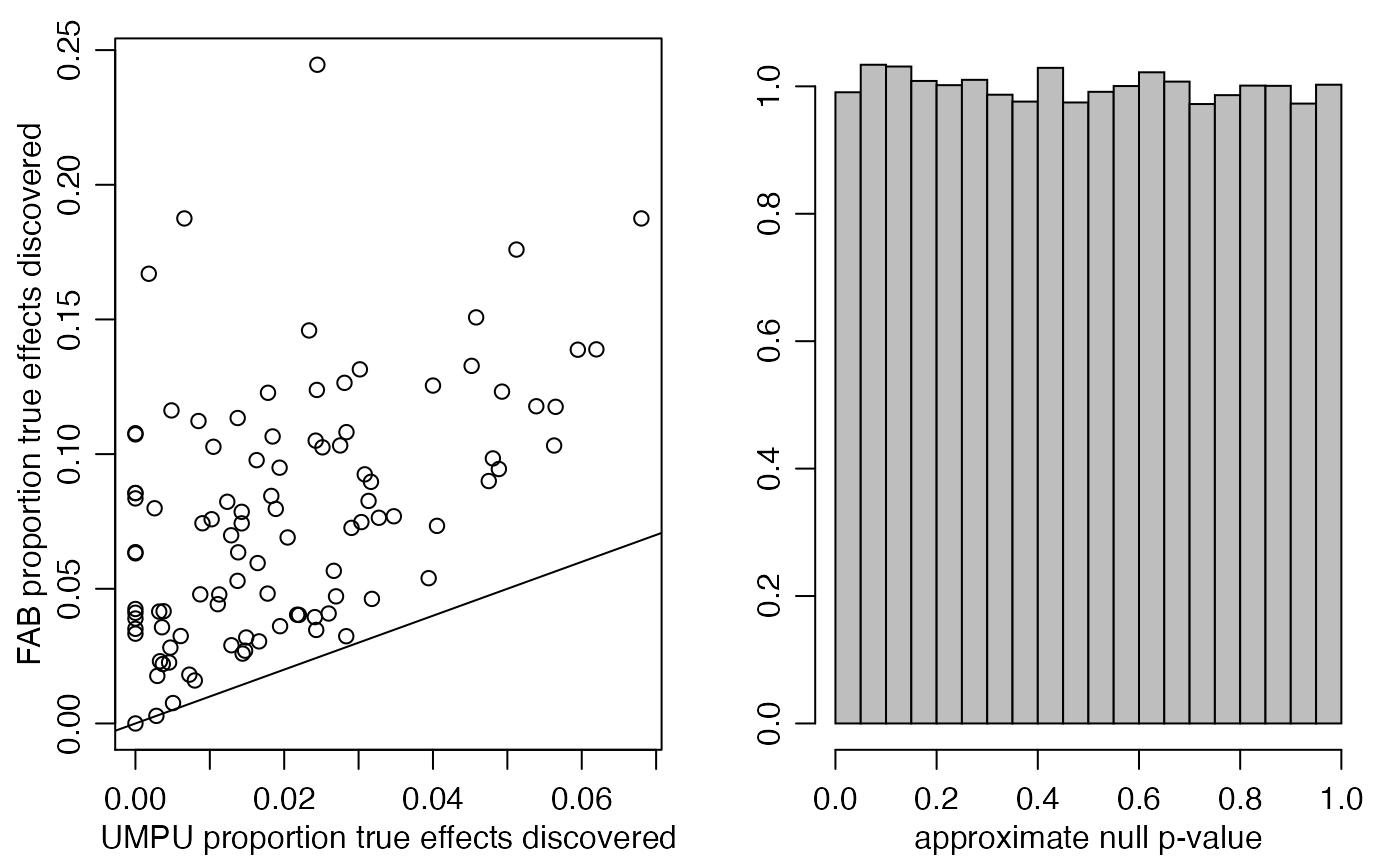
round(mean(UPOW),3)

## [1] 0.02

round(mean(EPOW),3)

## [1] 0.077

mean(EPOW)/mean(UPOW)

## [1] 3.851542

Plots:

par(mfrow=c(1,2),mar=c(3,3,1,1),mgp=c(1.75,.75,0))
plot(UPOW,EPOW,xlab="UMPU proportion true effects discovered",
               ylab="FAB proportion true effects discovered")
abline(0,1)

hist(pXNULL,main="",xlab="approximate null p-value",ylab="",prob=TRUE,
     col="gray")

Peter Hoff

2019-07-23

Summary